Introduction

There’s an interesting video on finding the average shadow of a cube. The video has a simple problem, a brute force solution, and finally an elegant closed form solution. Let’s find a problem with a similar situation and work through the steps.

Problem

Say that we are starting a collection and want at least one of every type. There’s a uniform probability of acquiring any such item. For n unique items, what is the expected number of samples until at least one of each collectible is obtained?

Brute Force

First, let’s write a program to try it out. When one of each collectible is chosen, return the number of samples to get there. Repeat this process to approximate a true solution. This code can be seen below. Note that the collectibles will be represented as unique integer values. And the collection is represented as a set.

static constexpr int kNumSamples = 1000000000;

double arithmetic_mean(const std::vector<int> &all_num_samples) {
    const int64_t sum =
        std::accumulate(all_num_samples.begin(), all_num_samples.end(),
                        static_cast<int64_t>(0));
    return sum / static_cast<double>(all_num_samples.size());
}

int compute_num_samples_to_fill_at_least_one_bin(const int num_bins) {
    static std::default_random_engine random_engine;
    int samples = 0;
    std::unordered_set<int> bins;
    std::uniform_int_distribution uniform_dist(0, num_bins - 1);
    while (static_cast<int>(bins.size()) < num_bins) {
        const int new_bin = uniform_dist(random_engine);
        bins.insert(new_bin);
        ++samples;
    }
    return samples;
}

double compute_num_samples_to_fill_at_least_one_bin_mean(const int num_bins) {
    std::vector<int> num_samples;
    for (int sample = 0; sample < kNumSamples; ++sample) {
        num_samples.push_back(
            compute_num_samples_to_fill_at_least_one_bin(num_bins));
    }
    return arithmetic_mean(num_samples);
}

Running a program over a range of values for some time may yield a plot like below.

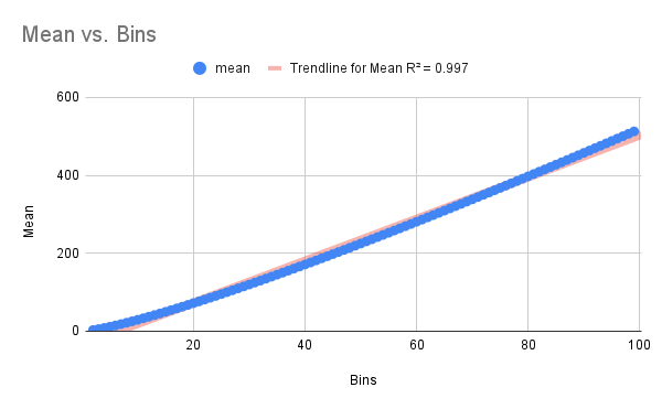
That looks promising. There’s clearly a trend, but it isn’t quite linear.

Steps Towards an Analytical Solution

Visualizing Every Brute Force Outcome

Below is a visualization of the various outcomes at each sample. Note that the shading level groups results with the same sample count. The area of the shading represents the probability of the result. Also, note that some of the results don’t terminate.

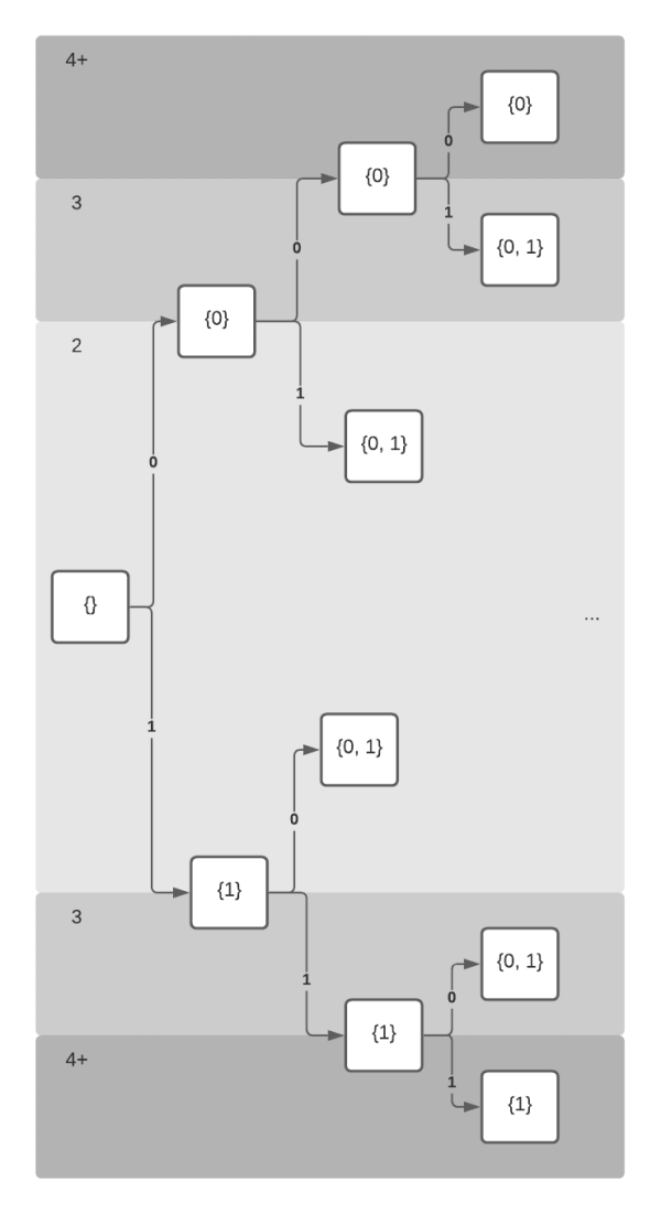
50% of the time it takes two samples to complete the set. 25% it takes three turns. And 25% it takes four or more samples.

Bounding the Long Tail

The space can be bounded by using the geometric series. The following equation computes the expected number of counts, when only one collectible is obtained and there are a total of two collectibles.

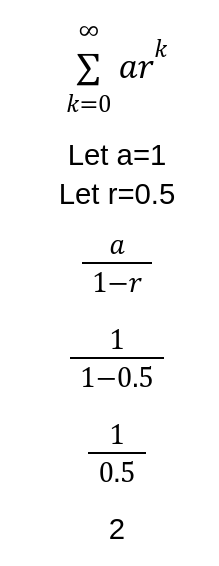
This equation is the same as determining the expected number of flips until heads on a fair two sided coin. As an equation, it might look like the following.

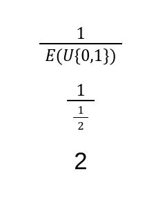
With the bounds, the chart looks like below.

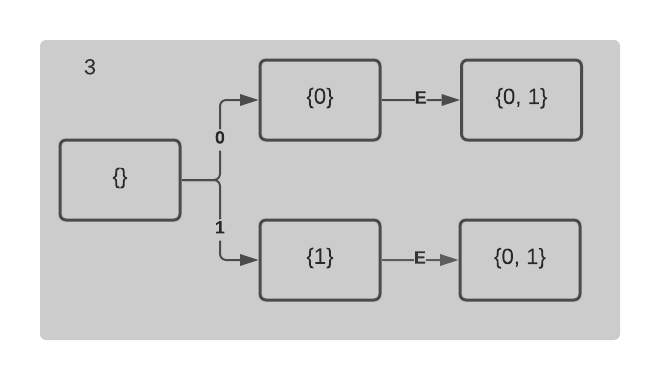
This chart is greatly simplified. After collecting unique item zero, there are two more expected samples to complete our collection. There’s a similar situation after collecting unique item one. So for two unique items, three samples are expected to complete our collection.

Observing Symmetry

The final step to achieving an analytical solution is to observe the symmetry among all the paths. It turns out that the order that the collectibles doesn’t really matter. What really matters is the number of unique collectibles obtained. Therefore, the sample chart isn’t a tree, but a list as shown below.

Furthermore, the order that the unique collectible is obtained doesn’t matter. Every step can be computed independently. Then, the final result can be added together in any order.

If we set the number of bins to n, we can say that the following equation computes the expected number of samples until all of them are chosen at least once.

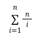
The previous equation is pleasing because it can be represented with only a few characters. Also, it can be computed accurately and efficiently for larger numbers.

Representing the Equation in Code

The previous equation can be represented as the following C++ code.

double compute_num_samples_to_fill_at_least_one_bin_analytic(
    const int num_bins) {
    double output = 0.0;
    for (int i = 1; i <= num_bins; ++i) {
        output += static_cast<double>(num_bins) / i;
    }
    return output;
}

In newer versions of C++ it may be possible to use ranges to express this in a more functional way. For example, there’s supposed to be a sum function in C++23. Unfortunately, as of writing this, it doesn’t exist in GCC. ranges v3 can get us pretty close. See below.

double compute_num_samples_to_fill_at_least_one_bin_analytic_ranges(
    const int num_bins) {
    auto n_div_i = [num_bins](const int i) {
        return static_cast<double>(num_bins) / i;
    };
    return ::ranges::accumulate(
        std::views::iota(1, num_bins + 1) | std::views::transform(n_div_i),
        0.0);
}

Using GCC 11.2, the ranges solution can generate similar code to the raw loop in terms of instructions with O2: godbolt. Take this measurement with a grain of salt. Ranges is new. There may be extra compile time overhead. In addition, there may be runtime overhead if parts don’t get optimized. One advantage to ranges is that the operation could be parallelized.

Conclusion

For a certain range of values on this particular problem, a linear fit model might be acceptable. The trend is a little harder to fit for large ranges. See the plot below for large numbers. Note that there is a log scale for both axes.

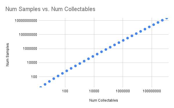
Computers are a great tool to hammer through a lot of math. Then, we can analyze those results to spot trends. Iterating on this process can produce elegant results. The result can feel victorious!